Planning with cost maps

Introduction

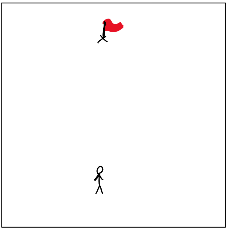
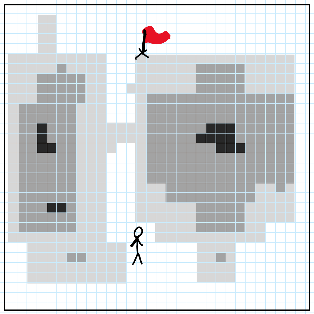
Imagine you’ve been asked to find the best path to the flag. Using the information given above, the answer obviously looks like this:

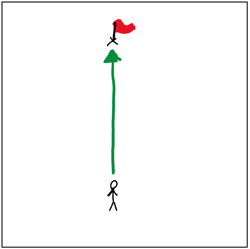
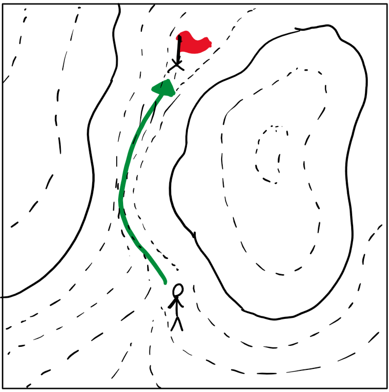
But what if we were given some additional information? If we add elevation data, the “best” path becomes the flattest one, since it takes the least effort:

To us, this solution is intuitive. In fact, most animals can select the optimal path to a goal without even thinking about it.

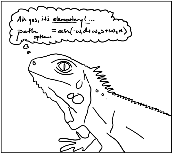
For example, imagine an iguana has just spotted a tasty fly. In finding the best path to this morsel, the iguana uses its beady eyes to scan the world around it, observing the locations of any possible predators and maximizing its distance ($d$) to each. It might prefer a path in the warm sun, so it avoids shady regions ($s$). Finally, to keep the element of surprise, the iguana avoids walking crunchy, noisy surfaces ($n$).

Our iguana, this prehistoric, cold-blooded creature, has just performed a multivariate optimization without so much as blinking: $path_{optimal} = \min(-w_1d+w_2s-w_3n)$, where $w$ is a weight for an individual factor.

If it’s so simple that a lizard can do it instinctively, then surely our car can plan paths in this fashion– right?

Let’s try dividing the map into cells. We can then assign each cell’s value to be the height at the cell’s center. Below we’ve discretized (categorized) the elevation into four values, but in our actual software, we use over 100 different values.

Next, let’s generate five paths randomly, stopping each path’s generation when it reaches some distance from the goal. We then select the path where the sum of each intersecting cell’s value is smallest.

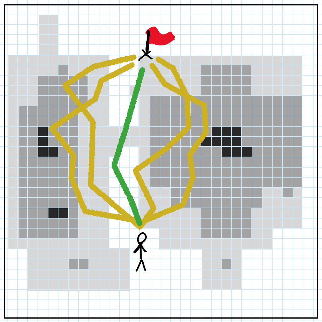
In the above example, we’ve generated just five paths. In reality, we might generate hundreds or even thousands. We can further optimize this by create a tree, where multiple paths may start from a common branch.

The real power of this grid-based approach is that each cell’s value can be calculated using multiple factors. Thinking back to the iguana, each cell’s value can be the weighted sum of sunniness, noisiness, and distance from predators.

Application to autonomous driving

Our upstream software already provides us with plenty of perception data: the location of curbs, pedestrians, cyclists, even fire hydrants. Our mapping and localization systems tell us exactly how far we are from the route, from the lane center, and the speed limits of each map region.

See where this is going? Using the factors provided by upstream nodes, we can generate a grid-based map of our vehicle’s current surroundings, then plot our goal on this map. Using the wealth of perception data already available, we assign each cell a cost, which is a big weighted sum from individual factors.

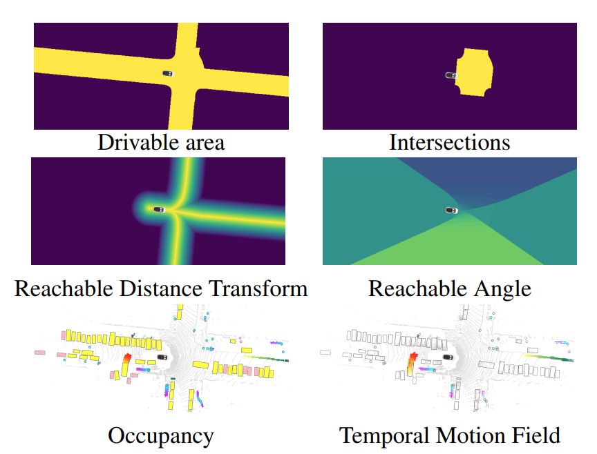
Instead of sunniness and noise, we now consider distance from the lane center, a cell’s class as either road or not-road, the lane’s speed limit, whether or not a cell is currently occupied, whether we predict it to be occupied in the near future, and so on.

We take inspiration from “MP3: A Unified Model to Map, Perceive, Predict and Plan” by Casas, Sadat, and Urtasun. Below are some figures from their paper:

We can take the weighted sum of the above values to produce a holistic cost map, a grid map that represents the complete cost of a robot’s choices. We can then apply a number of generative planners, such as Rapidly-Exploring Random Trees (LaValle ‘98), to find an optimal or near-optimal path.

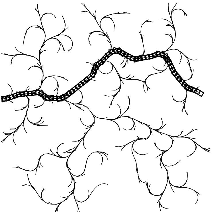
Above: An example rapidly-exploring random tree, from LaValle ‘98.