Getting Things Rolling With Demo 1

Getting started with autonomous cars can be scary. How do you start? We started in January with a simple goal: Travel from Point A to Point B. Every other factor would be simplified as much as possible. This led us to the following assumptions:

• Driving will occur in daytime, in good weather.
• A human will be behind the wheel at all times, ready to take over.
• This person will control the throttle and brake.
• The computer can only move the steering wheel.
• The computer will have access to processed, pre-recorded map data.
• The computer will be given its initial location and its goal location before it starts the trip.

We also defined a clear success condition, where all of the following are met:

• The car should travel from Point A to Point B.
• Only the computer should apply any control whatsoever to the steering wheel for the duration of the trip.
• The car should remain in the appropriate lane.

Finally, to meet the above criteria, we outlined five questions that demanded our attention:

1. What does the map look like?
2. Where am I on the map?
3. Where is my destination on the map?
4. What is the best path from my location to my destination?
5. How can I translate this path into steering angles?

Breaking our goal down into these five questions made things more clear and approachable.

Tools we used

Software

We’re lucky that a number of autonomous car “platforms” are publicly available for for researchers to use. These platforms offer implementations of popular algorithms for tasks like mapping and control. Platforms include openpilot, apollo, and a few others. But don’t be fooled like I was– using this software isn’t as easy as downloading a file and running it. Integration is an arduous process, no matter what platform you choose.

We ultimately decided to use Autoware.Auto. Autoware is a really transparant and easily extensible platform to adopt. It runs off a popular framework called the Robot Operating System, or ROS. Adding features on top of Autoware is as simple as writing our own ROS “node”.

Electronic Steering and CAN

To steer the vehicle programatically, we used an EPAS system provided by DCE Motorsport. The system includes a powerful motor that fits around the car’s steering column. It also includes a simple computer called an “ECU” that controls the motor.

To send our commands from our onboard computer to the EPAS ECU, we used a CANable Pro. All modern cars use CAN to send data to and from components– signals to turn on the blinkers, honk the horn, and so on. The CANable allows us to connect to our car’s CAN network and send steering commands over it, which the EPAS then receives.

On-board computing

We used an NVIDIA Jetson AGX Xavier to run our entire stack. We didn’t optimize our code to run efficiently on the Xavier’s GPU, but we still achieved decent performance.

The Xavier is power efficient, which is an important consideration since our vehicle’s batteries aren’t limitless. Strapping a big GPU workstation to the roof would not have worked.

Simulation

We tested our code in a simulator before testing on the car. We used the SVL Simulator, which can generate highly realistic environments. We ran all of this on a local server.

A nice thing about our code is that it doesn’t care whether it’s run in the simulator or on the real car. Our software’s only real-time inputs are the Lidar streams, which are provided by the simulator in the same way that they are by the car.

1. What does the map look like?

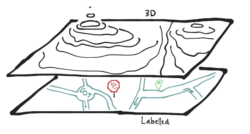Our map is split into two parts: A 3D map and a labelled map.

In the 3D map, a driver manually drives through the unmapped area and collects data from the car’s Lidar sensors. The data is then stitched together into a unified map file in a process known as SLAM. 3D maps are great at describing the texture of an environment. We can line up our 3D map with real-time Lidar streams later on, and that provides us with an accurate location estimate. 3D points combined together are often called “pointclouds”, so we commonly refer to 3D maps as “pointcloud maps” or “PCD maps”.

The labelled map gives context to our 3D data. Without it, a street curb is indistiguishable from a speed bump. The vast majority of labelled maps, including ours, are labelled by humans. These maps provide the location of stop signs, crosswalks, and traffic lights. They can store speed limits, road closures, even the locations of soccer fields. Most importantly, the labelled map tells us where lanes are located and how they’re connected. In other words, this map describes the road network. Examples of labelled maps include Google Maps and Open Street Map. Our maps use a specific format provided by the “Lanelet” library, so we refer to our labelled maps as Lanelet maps.

When we combine the pointcloud and Lanelet maps together, we create a rich description of our environment. This pointcloud-Lanelet double whammy is often called an “HD” map.

2. Where am I on the map?

Researchers call this problem “localization”. The most popular localization tool for everyday use is GPS (broadly called GNSS). GPS is not accurate or reliable enough for autonomous cars. Instead, most algorithms take GPS data as a starting point, then refine things with other data (usually LIDAR, stereo cameras).

We use an algorithm called Normal Distribution Transforms (NDT) to refine an initial location guess into an accurate result using real-time Lidar data and our 3D map. Specifically, we use Autoware.Auto’s implementation of NDT. Find more in this Autoware lecture. The original NDT paper is available here.

The basic steps of NDT are:

1. Divide our prerecorded 3D map into a uniform grid.
2. For each cell in our grid, calculate the average of all the points, along with the covariance. This makes our map much less complex, while still providing general information on how the points are dispersed within the map.
3. Take a real-time Lidar feed from the vehicle and place it onto our map using an initial guess (supplied by a passenger in Demo 1’s case).
4. Move our placed points around until they line up well with our grid of covariances (our processed 3D map).
5. Once our points are aligned, since we know where we are relative to our lidar feed (we’re in the center of the feed) and where our feed is on the map, we then know where we are on the map.

3. Where is my destination on the map?

This one is simple. Since we already have a map from #1, passengers just select a point on the map. This point is stored at our goal pose.

4. What is the best path from my location to my destinaton?

Imagine you’re looking for a restaurant that your friend told you about, and you’ve gotten lost. You stop and ask for directions, which are something like, “Go down McKinney Road, then turn right on Rose Parkway, then turn left on…” These general directions, just a sequence of streets to take, is generally good enough for humans.

In Voltron, we use a route planner to calculate this sequence of streets using our Lanelet map. It basically generates a sequence like a human would, like [McKinney Road, Rose Parkway...]. But this isn’t specific enough for computers. We need to refine these general directions into an exact line (curve) that the car follows. This refinement is done by our path planner.

We make the following distinction between “route” and “path”: routes provide general directions while paths are exact curves for the car to drive along. Paths can easily adapt to, say, drive around potholes.

5. How can I translate this path into steering angles?

At this point we know our current location (from #2) and the path we’d like to follow (from #4). We feed this information into a steering controller that turns this data into a steering angle.

Once we have our target steering angle, we feed it along with our current steering angle into a low-level PID controller. This calculates how much torque to apply to the steering wheel (literally how hard to turn the wheel, and it what direction). Finally, we translate this into a command to send to the steering motor. That’s it!