System overview
Maintained by Daniel Vayman
Table of contents
Design
Navigator is designed to be:
- Simple, with components that are easy to use an extend
- When a more powerful but complex algorithm is used, a simpler alternative should also be present
- Modular, with nodes that can be swapped, added, and updated with the help of ROS2
- Since nodes are all built using standard C++ and Python libraries, code is future-proofed.
- Open source, with all of our code licensed under the highly permissable MIT license
- Our dependencies are also open-source
About nodes and topics
Navigator is built upon ROS2, a communications framework where individual executables called “nodes” exchange messages through “topics.” A node can either subscribe to a topic or publish to it. In this fashion, individual nodes form a dense network where everything from camera streams to steering commands are passed from one node to the next.
Nodes can be grouped into packages. Packages are then grouped in workspaces. Navigator itself is a ROS workspace. It contains many packages, and each package contains at least one node.
Using ROS2, one node can gather raw LiDAR data from a sensor, where it publishes the pointcloud as a PointCloud2 message to a topic called /lidar/raw. Another node can then subscribe to /lidar/raw, filter the data, and publish the result to /lidar/filtered.
To learn more about ROS, watch this lecture by Katherine Scott, a developer advocate at Open Robotics.

Subsystems
We can divide Navigator’s nodes into five groups.
The perception subsystem interfaces with our sensor hardware (Lidars, radar, cameras, IMU, etc), handles any formatting and filtering, and publishes that data for our planning subsystem. This subsystem also handles object detection, classification, and tracking. Some types we use here are Image messages, PointCloud2 messages, Imu messages, and so on. We also produce OccupancyGrid and other cost map messages as an insightful tool for path planning.
The prediction system uses our perception output to predict future events. We use machine learning models, either pre-trained our trained in-house on our server, to achieve accurate, insightful, and usable prediction data. Some examples of what we’d predict are position of nearby vehicles, parking lot behavior, lane mergers, and pedestrian/VRU actions.
The mapping systems holds any nodes we use for mapping, routing, and localization. We pull geometry from pre-drawn, local map data to output routes, waypoints, and cost maps for use by our planning subsystem. While we currently rely on our nifty GNSS RTK hardware for precise localization, we plan to implement Simultaneous Localization and Mapping (SLAM) as an algorithmic solution.
The planning subsystem takes our perception and mapping results and decides what our vehicle should do. This subsystem handles both high-level decisions (Should we pass a car that’s stopped in the road?) and low-level ones (How far should we press the throttle pedal to reach our desired speed?). Our path planner traverses our cost maps to form precise trajectories.
The controls subsystem is the link between our software and hardware. It includes nodes that communicate with our steering hardware, our microcontroller, and more. Both the perception and controls subsystems, specifically the nodes in our vehicle_interface repository, are vehicle-specific, which means that they need to be configured to suite each individual vehicle. At Nova, we have separate configurations for simulated driving and real-world use.
Cost maps
During execution, Navigator calculates several cost maps, which are grid-based maps of our surrounding area that describe where our car should or should not drive.
Each cell in the grid is assigned a cost. The higher the cost, the less likely our car will generate a path that moves through the cell. This results in paths that weave their way through only low-cost cells. If no low-cost cells are available, the car stops and waits.
We calculate and use multiple cost maps, each one representing a unique factor to consider. For example:
- Our occupancy grid generator describes the location of objects (cars, people, curbs).
- Our prediction network (PredNet) node describes the future location of obstacles.
- Our red light detector marks intersections as high-cost regions if the light is red.
- Our map manager assigns costs based on how far a cell is from the route and from the goal.
We add as many of these layers together to form a single, holisitic costmap that our motion planner uses as its input.

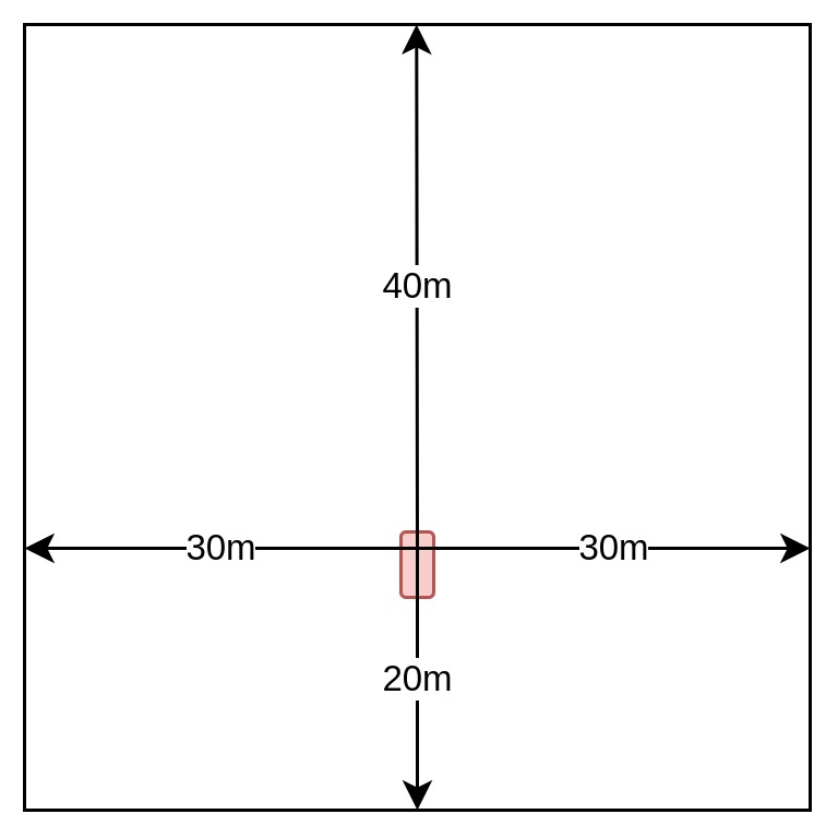
Above: Cost map dimensions
Cost maps should be in the base_link (vehicle) reference frame. They should extend 40 meters in front and to the side of the car and 20 meters behind, forming a total area of 80 x 60 meters. Cells should have a side length of either 0.2, 0.4, 0.8, or 1.6 meters.

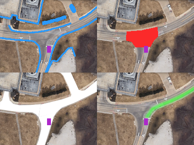
In the above example, each image is 200 x 150 pixels, representing a cost map layer with a resolution of 0.4 meters/cell. Clockwise from top left: Current occupancy, junction cost (due to a stop sign), route distance, and drivable area.